


Tom Brady is projected to have 25 completions, is over 23.5 -130 a good bet?
LeVeon Bell is projected to have 90 rushing yards, is over 102.5 +160 a good bet?
These are the questions we will answer in this article. As a starting point, we need to come up with a definition of what makes “a good bet”.
EV and +EV
To analyze any bet, we need three pieces of information – a list of all possible outcomes, a result (or payoff) for each one and a probability for each one. We can illustrate with the simplest possible bet – a coin flip.
Example #1: A common Super Bowl prop bet is the coin flip: heads -105, tails -105. Is heads -105 a good bet?
Here are the three pieces of information we need to analyze this bet. Let’s say we placed a $1 bet on heads.
Result is Heads: + $.952, probability 50%
Result is Tails: -$1, probability 50%
Now, let’s introduce a concept called expected value (EV for short). EV is calculated using a two-step process:
Step 1: For each outcome, multiply the result by the probability.
Step 2: Add up all of the numbers from step 1.
Result is Heads: result*probability = .476
Result is Tails: result*probability = -.5
.476 + -.5 = -.024
So the EV of this Heads bet is -$0.024 per $1 bet, or -2.4% of the amount bet. What does this mean? It does NOT mean that you are predicted to lose $0.024 on this bet (that is clearly impossible, you will either win $0.952 or lose $1.00!) It means that if you were to repeatedly make this same bet over and over again and accumulate your results, eventually the ratio of your total amount won/lost to your total amount bet would get very close to -0.024.
Why do we care about EV? Because over the long term, any bettor will experience a combination of good luck and bad luck that will balance each other out over time, so that all that’s left over is the EV. Most gambling propositions have negative EV for the bettor, allowing the entity offering the bet to make a profit – this is also known as the house edge, the vig or the rake.
Now, let’s look at a slightly different example.
Example #2: Coin flip: heads +108, tails -118. Is heads +108 a good bet?
Result is Heads: + $1.08, probability 50%, result*probability = .54
Result is Tails: -$1, probability 50%, result*probability = -.5
.54 + -.5 = .04
This time the EV is +0.04 per $1 bet, or +4%. If this bet is repeated over and over again, over a long enough time period that the good luck and the bad luck even out, the bettor will be left with a net win approaching $0.04 per $1 bet. It logically follows that any bet with positive expected value, or +EV, is a good bet.
Now, let’s use this “+EV” decision rule to evaluate some common NFL props.
Example #3: Tom Brady is projected to have 25 completions, is over 23.5 -130 a good bet?
Result is o23.5: + $.769, probability ?%, result*probability = ?
Result is u23.5: -$1, probability ?%, result*probability = ?
? + ? = ?
We quickly run into a problem – we don’t know the probability of over/under 23.5 completions. All we have is the projection of 25 completions – a number that is related to, but not quite the same as, what we need. It’s time to add something new to our toolbox.
Introduction to Probability Models
Let’s take an unknown quantity like “Tom Brady’s number of completions”. We can ask ourselves many different questions about this quantity. For example:
- What is the expected (or average) value of the # of completions?
- What is the probability of exactly 24 completions?
- What is the probability of over 23.5 completions?
- What is the probability of an odd number of completions?
- Etc, etc, etc.
We can think of a probability model as a “master key” that can unlock the answers to all of these questions. It works by assuming that a certain mathematical relationship exists among the probabilities of each possible outcome (known as the “probability distribution”). If we can define the probability distribution for an unknown quantity, we have our master key.
Simple Probability Models – The Poisson Distribution
For our investigation into Tom Brady’s number of completions, we turn to one of the simpler probability models – the Poisson distribution. In order for Poisson to apply, all of the following conditions must be satisfied:
- The unknown quantity in question must be a count of the number of times an event occurs (in this case, Brady completing a pass) over a given period of time.
- The events must be independent of each other; that is, Brady completing a pass doesn’t change the likelihood of him completing the next one.
- The likelihood of the events occurring must be consistent across the time period (i.e. Brady has the same likelihood of completing a pass in the 1st quarter vs the 4th quarter, the 1st minute vs the 60th minute, etc).
Footnote: The astute reader may notice that none of these conditions are entirely satisfied in the example of Brady’s completions. A game may be 60-75 minutes of playing time depending on overtime. A completed pass generally lengthens the time the Patriots offense is on the field, providing opportunities for more completed passes. Brady will be less likely to attempt passes in the 4th quarter if the Patriots are leading (which they usually are). While these are all true, the “close enough” rule applies here – none of these violations are significant enough to make me abandon the simplicity of Poisson in favor of some other, much more complicated probability model.
The neat thing about Poisson is that the expected (or average) value IS the master key! So if we interpret the projection of 25 completions as an expected value, we have everything we need.
Now, let’s use this master key to unlock the probability of over 23.5 completions. The bad news is that this requires a mathematical formula that would bring tears to the eyes of people who still have nightmares about their high school algebra classes. The good news is that there are plenty of software tools that can do the math for you. For example, the Microsoft Excel formula to calculate the probability of an unknown quantity being UNDER a given number is:
=POISSON.DIST(<number>,<expected>,TRUE)
For our Brady calculation, =POISSON.DIST(23.5,25,TRUE) gives a result of 0.394. Remember, this is the UNDER probability – to get the OVER probability, take 1 – 0.394 = 0.606 or 60.6%. Now we can finish the EV calculation:
Result is o23.5: + $.769, probability 60.6%, result*probability = .466
Result is u23.5: -$1, probability 39.4%, result*probability = -.394
.466 + -.394 = .072
The result of +0.072 per $1 bet means that a bet of Over 23.5 completions at -130 is indeed +EV and, therefore, a good bet.
Other prop bets where Poisson can be used:
- Over/under # of pass receptions
- Over/under # of rushing attempts
- Over/under # of touchdowns (for a team or a player)
- Over/under # of field goals
- Over/under # of penalties
- Will QB throw an interception Yes/No? (This can be re-stated as “Over/Under 0.5 interceptions”)
The Longest Yard(s)
Example #4: LeVeon Bell is projected to have 90 rushing yards, is over 102.5 +160 a good bet?
Note that props involving passing yards, rushing yards and receiving yards do not appear on the list above. That’s because they violate condition #1 of the Poisson distribution – they are not a count of how many times something happens. So Poisson, if we were to apply it, would give an incorrect answer.
For yardage props, there is no probability model that is as clearly applicable or as computationally simple as Poisson. In my own analysis, I have chosen to use something called a Compound Poisson model that has two components – a Poisson distribution for the number of completions / receptions / rushing attempts, and another distribution (I’ve selected a Gamma distribution) for the number of yards gained on each.
This distribution does not fit into a form that is easily calculable using a simple formula. Instead, I’ve created these lookup tables that you can use, the left is the yards that you are expecting or projecting and the top is the probability of exceeding it:

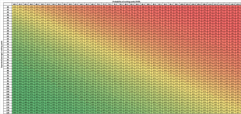

The first things you may notice when looking at these tables are some counter-intuitive results in the center of them. For example, a receiver with 70 expected receiving yards has only a 44% chance of going over 70.5, and only a 49% chance of going over 66.5. Don’t tweet me about an error in the table – there isn’t one! This is a statistical phenomenon called “skewness” and it happens for the following reason: Suppose DeMarco Murray is projected for 70 expected rushing yards. There is a chance (a small chance, but a chance) that he has a phenomenal game and exceeds his expected total by 90 yards, giving him a 160 yard rushing game. There is NO chance for him to fall short of his expected total by 90 yards because that would result in a -20 yard rushing game and that is impossible (yes, I know it’s technically possible to have negative rushing yards but this type of model does not consider negatives). Because these extreme outliers are prevalent on the over side and not on the under side, they “skew” the average – causing it to be a little bit higher than the median (i.e. the number where there is a 50-50 split between over and under).
Now let’s return to the example of Le’Veon Bell over 102.5 +160. We need to look at the rushing yards table. In the row for 90 expected rushing yards and the column for over 102.5 rushing yards, the value is 33%. This is the probability of over 102.5 rushing yards, which we can plug into our EV calculation:
Result is o102.5: + $1.60, probability 33%, result*probability = .528
Result is u102.5: -$1, probability 67%, result*probability = -.67
.528 + -.67 = -.142
The EV is -0.142 per $1 bet, or -14.2%. Because the EV is negative, this is NOT a good bet.
Conclusion
I hope you have enjoyed this introduction to how the EV calculation can be used to identify good bets, and how probability models can be used as “master keys” to unlock probabilities for some of the most common types of NFL prop bets. In my next article, we will dive into the Kelly Criterion and how to take the best possible advantage of +EV bet opportunities to maximize your long-term bankroll growth.
Tweet me with any comments or questions at @PlusEVAnalytics. Until next time, may your EV be positive and may your variance be favorable!